Belmont's public coyote map is the kind of thing that dares you to overinterpret it. The points are visibly uneven. They look denser in some parts of town than others, especially toward Belmont's greener western side. If you were moving quickly, you could look at that map and say: there, that's where the coyotes are.

That is exactly the temptation this post is trying to resist.

Opportunistic wildlife sightings are not telemetry. They are not a census. They are not a uniform sample of animal locations. They are a human reporting process laid on top of an animal process. A cluster of reports can mean more coyotes, more people noticing coyotes, more people willing to file reports, repeated reports from the same vantage point, or some combination of all of those.

Belmont's data are unusually useful because the public map exposes enough structure to let us test some of those possibilities directly. We can recover the point geometry, report date, report time, and reporting address. We cannot identify reporters by name, and we cannot read narrative notes. So this is not a detective story about proving a literal super-caller. It is a spatial-analysis story about what kinds of clustering survive once we confront duplicate locations, repeated addresses, temporal concentration, and weak ecological controls.

My bottom line is careful but not trivial: Belmont's public coyote reports are clearly non-uniform in space, but the strongest interpretation supported here is non-uniform report concentration, not a clean map of coyote behavior. Repeated origins matter a lot. A simple habitat story is not well supported by the first-pass contextual tests. The right conclusion is a mixture, with reporting concentration carrying more of the evidentiary weight than habitat concentration in this version of the analysis.

The data we actually have

Belmont's public PeopleGIS viewer includes a Coyote Sightings layer. The town does not expose it as an easy one-click download, but the web app's own query endpoint returns a structured record set. Recovering that public payload yielded 290 reports with:

• point geometry
• reporting address
• report date
• time string
• internal record identifiers

What the public layer does not expose is just as important:

• no reporter identifier
• no narrative note text
• no explicit duplicate flag

That means the analysis can test for repeated locations and repeated addresses, but not for repeated named reporters. It also means every claim in this piece has to stay one step more modest than it otherwise might.

To put the reports in context, I joined the points to a Belmont town boundary and clipped in two official statewide context layers from MassGIS:

• protected and recreational open space
• National Wetlands Inventory wetlands

Those are useful first-pass context layers, but they are not an exposure-aware model of where people live, walk, or decide to report. That matters later.

Figure 1: the raw map already hints at the problem

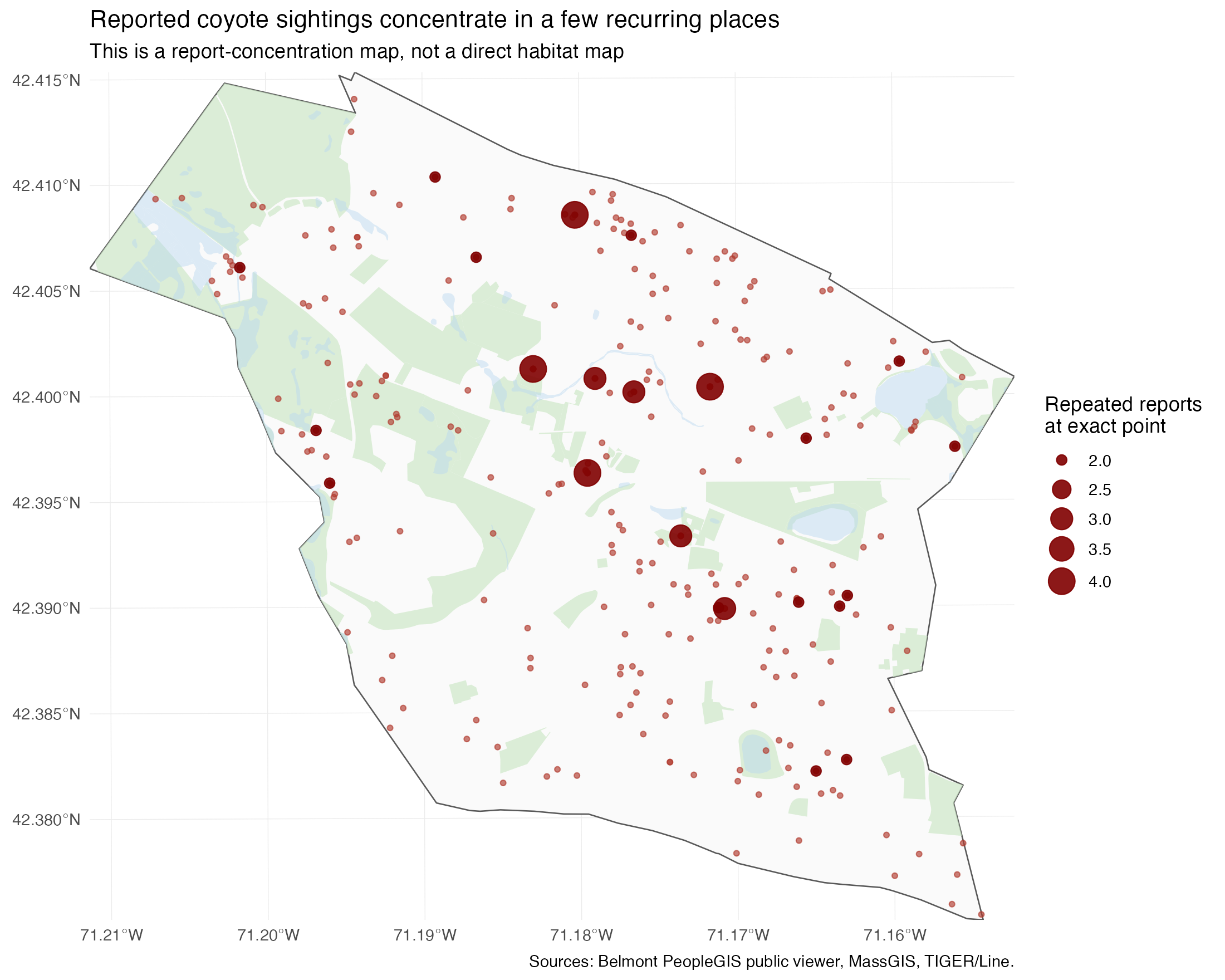
Figure 1. Raw Belmont coyote reports over Belmont boundary, open space, wetlands, and repeated exact locations. Larger dark-red symbols mark exact coordinates that appear more than once.

Figure 1 is the obvious starting point. The reports are not spread evenly across Belmont. But just as important, some places recur. The larger dark-red points show exact coordinates that appear repeatedly in the public archive. That is the first reason not to read the map as direct habitat telemetry. The same mapped place can contribute multiple reports over time.

Even visually, this is a mixed signal. There is some western-side concentration, but there are also central and south-central reports. And the repeated points are often on ordinary residential streets, not just on the edges of mapped open space. So before doing anything more sophisticated, the raw map already tells us that two stories are plausible at once:

• a spatial pattern in where coyotes are encountered
• a spatial pattern in where people repeatedly observe and report them

The statistical setup

Because the audience here is data-science-y, it is worth being explicit about what was actually estimated.

The analysis pipeline treated Belmont as a bounded observation window and ran several complementary diagnostics:

1. Nearest-neighbor ratio against CSR For each scenario, I computed the mean nearest-neighbor distance among points and divided it by the expected mean nearest-neighbor distance under simulated complete spatial randomness inside Belmont. The ratio is below 1 when points are more tightly packed than the null. This is useful as a non-uniformity diagnostic, but here it is a test of report concentration under a uniform-placement null, not a clean ecological test.

1. Quadrat test Belmont was partitioned into a 4x4 grid and the count pattern was tested against uniform intensity. This is a blunt but interpretable test for uneven spatial counts. Again, in this setting it is a reporting-process benchmark more than a behavioral one.

1. Ripley's L I estimated Ripley's L and compared it to a Monte Carlo CSR envelope. This helps show whether the pattern is more clustered than CSR over a range of distances instead of at just one nearest-neighbor scale.

1. Kernel density estimation I fit a KDE using Diggle's bandwidth rule. KDE is descriptive, not dispositive. It can summarize where reports pile up under one smoothing choice, but it is not itself a causal argument.

1. Local Moran hotspot map I aggregated reports to a Belmont-clipped fishnet and ran local Moran's I. This is also descriptive and scale-sensitive. I explicitly saved a sensitivity table across 150 m, 250 m, 400 m, and 600 m grids because one hotspot map can easily look more definitive than it really is.

- raw reports - unique exact coordinates - a version with the five most repeated exact locations removed

1. Duplicate and repeat-origin diagnostics This is the real center of gravity of the piece. I compared:

I also summarized repeated reporting addresses, same-address same-day repeats, same-address same-week repeats, and addresses that map to more than one coordinate.

1. Ecological-context comparisons I compared unique sighting locations to random points inside Belmont using distance to open space and distance to wetlands, plus a simple logistic model on log-distance predictors. These are only first-pass diagnostics because the controls are not exposure-aware. A random point inside a wetland is not a realistic stand-in for a human reporting opportunity.

That setup matters because every conclusion below depends on what the null is. If you compare a human-origin reporting archive to uniform random points over all of Belmont, rejecting that null tells you the reports are not uniform. It does not tell you, by itself, that coyotes are choosing those exact places.

Figure 2: yes, the reports are clustered under a simple null

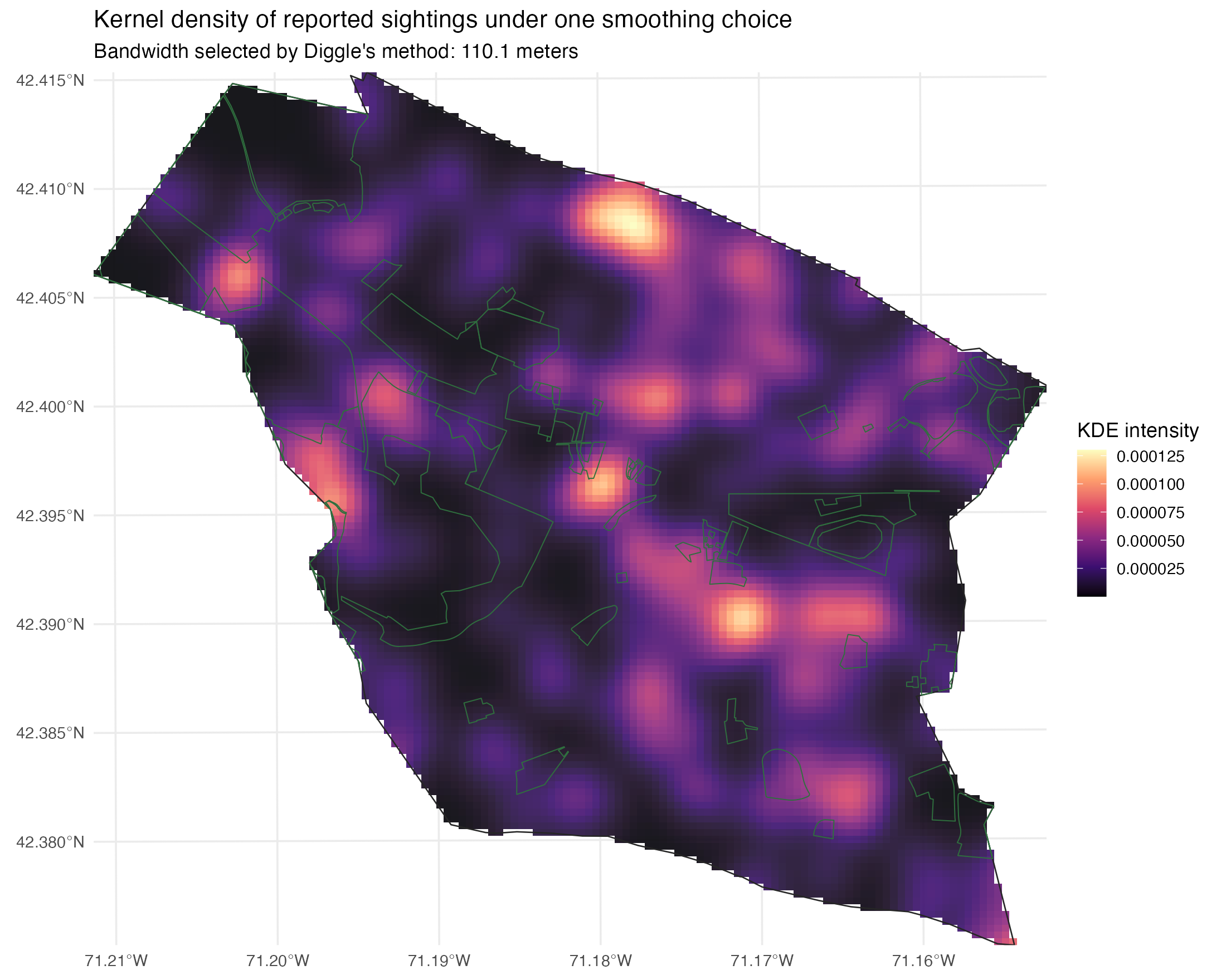
Figure 2. Kernel density surface for raw reports under one smoothing choice. This is descriptive smoothing of a reporting archive, not direct evidence of coyote habitat use.

Under a simple CSR benchmark, Belmont's reports are clearly non-uniform.

The main clustering results are:

• raw nearest-neighbor ratio: 0.697 with Monte Carlo p = 0.005
• unique-location nearest-neighbor ratio: 0.833 with Monte Carlo p = 0.005
• raw quadrat test p = 1.6e-07
• unique-location quadrat test p = 2.01e-05
• Ripley's L exceeds the CSR envelope in the tested distance range for all three scenarios saved in the output

So if the question is "are these reports spatially uniform over Belmont?", the answer is clearly no.

But that is only the first question. Figure 2 is useful because it shows where the archive looks dense under one smoothing rule. It is not useful as a shortcut to "this is where coyotes live." KDE will always make repeated and nearby reports look like a broad underlying surface, even when some of the structure comes from repeated origins.

There is a second complication too: the archive is pooled over a long time span. About 46.0% of the dated reports fall in 2011-2012 alone. So any all-years density surface is blending together different reporting eras as well as different locations.

Figure 3: repeated origins are not a side issue

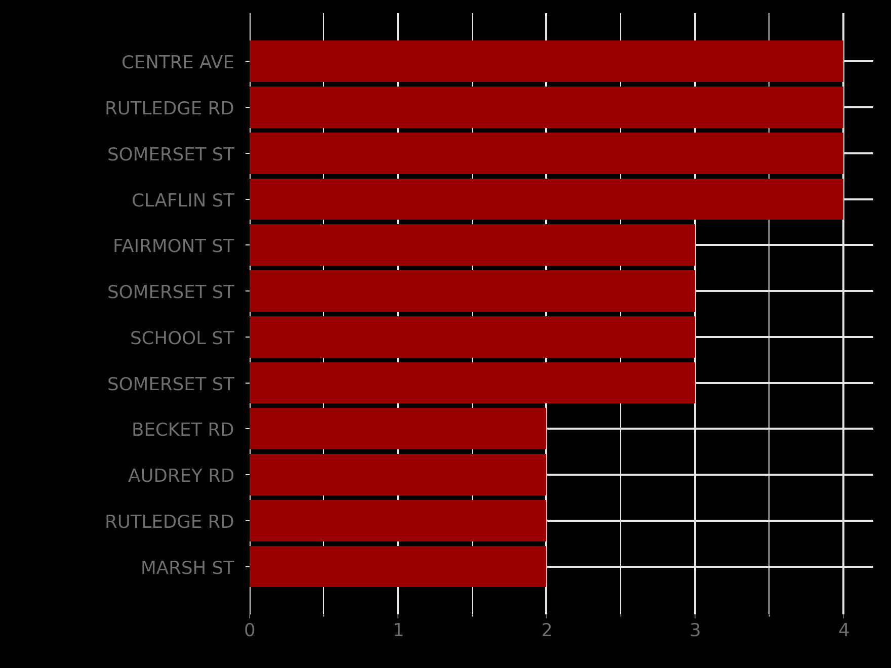
Figure 3. Top repeated report origins in the raw report set, with house numbers omitted from the labels for privacy.

If the whole map were being driven by one spectacular super-caller, the story would be easy. The public data do not let us prove that, and the evidence does not support that kind of dramatic claim anyway.

But Figure 3 shows something important and more defensible: repeated origins are common enough to materially shape the map. To avoid pointing readers at a specific household, the figure omits house numbers from the labels rather than printing the full addresses.

The duplicate and repeat-origin diagnostics show:

• 22.8% of all reports fall on exact coordinates that repeat
• 27.0% of nonblank-address reports come from addresses that repeat
• 25 reporting addresses appear at least twice
• 6 addresses recur in more than one mapped coordinate
• 5 same-address same-day repeat events appear in the public layer
• 6 same-address same-week repeat events appear in the public layer

That is not evidence of fraud, fakery, or one obsessive resident running the entire map. It is evidence that repeated report origins are structurally important. Once roughly a quarter of reports come from repeated exact points or repeated addresses, any naive heatmap interpretation becomes much too strong.

Figure 4: clustering survives deduplication, but it weakens

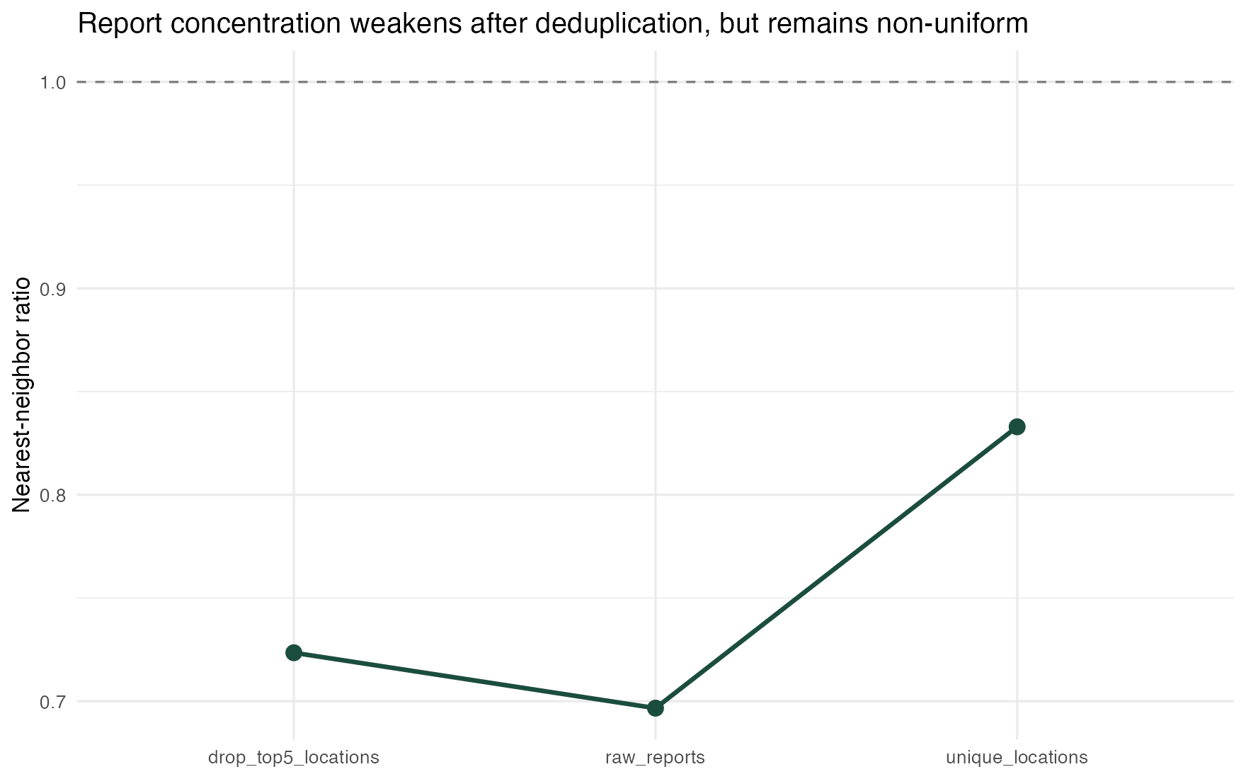
Figure 4. Robustness check using the nearest-neighbor ratio. Moving from raw reports to unique exact locations weakens clustering, but does not eliminate non-uniformity.

Figure 4 is the most important figure in the post.

The raw archive contains 290 reports, but only 251 unique exact locations. When repeated exact points are collapsed, the nearest-neighbor ratio moves from 0.697 to 0.833. That is still below 1. The pattern is still non-uniform. But the clustering gets less dramatic once repeated coordinates stop counting as independent observations.

That is the strongest clean result in the package:

• there really is spatial concentration in the reporting archive
• some of that concentration survives deduplication
• but the raw archive makes the pattern look sharper than it is

The top-five-location removal check points in the same general direction, though less cleanly across every metric. That is why the post now treats the robustness result as "clustering weakens" rather than "the truth emerges once duplicates are removed." Even after deduplication, the residual pattern could still reflect broader reporting opportunity rather than coyote behavior per se.

Figure 5: hotspot geography is descriptive and scale-sensitive

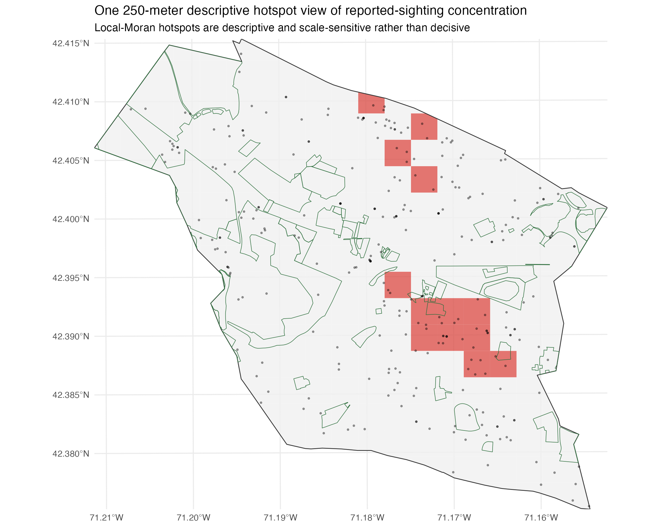
Figure 5. One 250-meter hotspot view of reported-sighting concentration. This map is descriptive; the hotspot footprint changes materially with grid size.

Figure 5 is useful, but only if it is read skeptically.

At a 250 m grid, the local Moran map suggests a concentrated set of report hotspots. But the sensitivity table shows how unstable that picture is across spatial resolutions:

• raw-report hotspot cells: 27 at 150 m, 13 at 250 m, 10 at 400 m, 6 at 600 m
• unique-location hotspot cells: 26 at 150 m, 12 at 250 m, 10 at 400 m, 3 at 600 m

That is not a stable hotspot footprint in the strong sense. It is a scale-dependent descriptive pattern. The map is still worth showing because it helps readers see how a municipal archive can generate visually compelling clusters. But the right interpretation is: here is one way the report concentration looks under one aggregation choice, not here is the true set of coyote hotspots.

This is also where the western-side story has to be handled carefully. Some maps do place more visual emphasis on Belmont's west side near Rock Meadow and other greener edge areas. But the same outputs also show central activity, and the hotspot footprint moves around with cell size. So the west-side read is a clue, not a settled result.

Habitat story or reporting story?

The first-pass habitat diagnostics are weaker than the maps make you want them to be.

When unique sighting locations are compared to uniform random points inside Belmont:

• median distance to open space is 138 m for sightings versus 99 m for controls
• median distance to wetlands is 277 m for sightings versus 251 m for controls
• the wetland comparison is weak statistically
• the open-space comparison actually runs against the simple idea that the reports cluster right next to mapped open space

That does not prove the western-edge story is wrong. It does mean the first-pass official layers do not strongly validate it.

There are two reasons to be cautious here.

First, the controls are weak. Uniform random points over Belmont are not a realistic model of where people encounter and report coyotes. An exposure-aware design would sample from places people plausibly observe from: residential parcels, address points, road frontage, or some other human-accessible background.

Second, "open space" is not the same thing as "coyote corridor." Coyotes may move along edges, backyards, informal green strips, cemeteries, rail-adjacent spaces, or other features that this first-pass context set does not capture well.

So the habitat-versus-reporting verdict is asymmetric:

• the reporting-bias evidence is concrete and fairly strong
• the habitat evidence is plausible visually but weak in the first-pass formal tests

What can we say about the super-caller hypothesis?

Not as much as a dramatic version of the story would like.

The public data do not identify reporters. So this analysis cannot prove that one household or one especially dedicated resident generated a large share of the archive. It also cannot prove that repeated addresses correspond to the same person over time.

What it can say is narrower and still important:

• repeated exact points matter
• repeated addresses matter
• repeated address-week combinations exist
• clustering weakens when repeated exact points are collapsed

That is evidence consistent with observer concentration. It is not evidence of a single dominant named reporter.

The safest phrasing is that Belmont's raw map looks more like a mixture of:

• a non-uniform reporting process
• repeat observations from recurring origins
• and possibly some underlying spatial structure in coyote encounters

with the current design unable to separate those cleanly.

A compact methods note for people who want the implementation details

The full workflow is in the exploration outputs, but the high-level implementation choices were:

• the public PeopleGIS query was scripted and saved as a raw JSON artifact
• point geometry was recovered and transformed into Massachusetts mainland meters for spatial analysis
• randomized procedures were seeded with set.seed(20260408) for reproducibility
• all main outputs were regenerated from a single R script
• robustness work compared raw reports, unique exact locations, and a top-repeat-removed variant
• time concentration was summarized separately because the archive spans more than twenty years
• hotspot sensitivity was tabulated across multiple grid sizes instead of relying on one map

If I were taking this into a second, stronger round, the next methodological upgrades would be:

1. build an exposure-aware background model
2. validate a few point locations directly against known addresses or landmarks as a stronger CRS audit
3. stratify or model the archive by time period instead of leaning so heavily on a pooled 2003-2025 surface
4. add richer context layers such as rail corridors, cemeteries, parcels, and street network structure

Side quest: weird Massachusetts municipal GIS

This project also turned up a sidecar catalog of other Massachusetts municipal GIS layers that deserve future attention. A few especially promising examples:

• Weston wildlife-reporting infrastructure
• Dedham's tree inventory and sewer infrastructure layers
• Cambridge's street-tree data

Those datasets are not the main event here, but they are a reminder that town GIS portals sometimes contain surprisingly rich raw material for small-scale empirical work.

Limitations

This entire analysis is built on opportunistic public reports rather than a controlled survey or animal-tracking data. The records are pooled across more than two decades. Reporter IDs and narrative notes are absent. The ecological controls are not exposure-aware. KDE and hotspot maps are descriptive and scale-sensitive. The geometry required CRS validation because the viewer metadata could not simply be trusted. And the context layers used here are first-pass rather than exhaustive.

Those are real limitations, but they are not fatal. They just determine what kind of claim this post is allowed to make.

The takeaway

Belmont's public coyote reports are clearly non-uniform, but that is not the same thing as a clean behavioral map of coyotes. The strongest evidence in this package is evidence about reporting concentration: repeated coordinates, repeated addresses, temporal bunching, and clustering that softens after deduplication. The habitat story remains possible, especially in a broad western-edge sense, but the first-pass formal context tests do not carry that story very far.

If you want the disciplined interpretation, it is this: Belmont's coyote map is informative, but mostly as a map of reported encounters shaped by both animal movement and human observation. The raw clusters are real as features of the archive. They are not clean proof of where coyotes "really are."

If you want the replication materials, code, intermediate outputs, and notes, they live here: analysis folder for this project. The main executable pipeline, including the public-data recovery step, is src/run_analysis.R.

• Gave an elections and redistricting project a more durable Codex workflow.
• Added clearer places for planning, review notes, and repeated research tasks.
• Put the first cross-project Codex diary system in place.
• The nightly summary now comes from saved breadcrumbs and git history, not chat memory.
• Cleaned up the personal academic website and blog for launch.
• Newer posts with images and numbered lists now render correctly.
• Tightened blog timing so the daily diary stays hidden until the evening.
• Wrapped up a Philip Roth text-analysis package for public release.
• A coyote-sightings analysis now makes a narrower claim about reporting clusters rather than animal behavior.

People ask for a Roth analogue as though the answer should be obvious. But "like Philip Roth" can mean at least five different things at once. It can mean writing about sex, guilt, family, ethnic inheritance, and American institutions in the same key. It can mean a certain sentence texture: tense, intelligent, restless, self-revising. It can mean the social choreography of his fiction: parents, lovers, rivals, intellectuals, doctors, campuses, Jewishness, class aspiration, urban and suburban pressure. Or it can mean something harder to pin down but impossible to miss in a good Roth novel: the voice that is forever confessing, prosecuting itself, justifying itself, and talking itself into the next trouble.

That is why the usual "if you like Roth, read..." lists always feel a little thin. They collapse several different likenesses into one word. Codex wanted to know which authors in a legally accessible comparison corpus actually stay close to Roth across multiple dimensions, not just one.

So Codex built a constrained but honest corpus and measured it.

If you want the replication materials, code, intermediate outputs, and notes, they live here: replication folder for this analysis. The key scripts are src/run_pipeline.py, which downloads the source pages and builds the corpus, and src/make_figures.py, which generates the figures.

The method, in plain English

The strongest local corpus Codex could legally and reproducibly access during this run was not a folder of full novels. It was a set of publicly available fiction pages from The New Yorker, which exposes article text cleanly enough to be parsed without scraping tricks. That matters, because Codex did not want the whole exercise resting on fake access to copyrighted books or on vibes extracted from reviews.

The final corpus included 46 usable texts and about 329,000 words from eleven authors: Philip Roth plus Don DeLillo, Jhumpa Lahiri, Zadie Smith, Mary Gaitskill, Jennifer Egan, Junot Diaz, George Saunders, Lorrie Moore, Aleksandar Hemon, and Tessa Hadley.

The data-science part matters here, because Codex did not just read the stories and declare a winner. Codex turned the corpus into numbers several different ways.

First, Codex split the texts into roughly 350-word passages and built a high-dimensional term matrix using TF-IDF on words and bigrams. Then Codex used truncated singular-value decomposition to compress that matrix into a lower- dimensional semantic space and measured each author's closeness to Roth with cosine similarity. That gave Codex a topic / semantic score.

Second, Codex built a stylometric feature table: average sentence length, sentence- length dispersion, paragraph length, lexical diversity, punctuation habits, dialogue density, and a function-word profile. Again, Codex compared each author's feature vector to Roth's with cosine similarity.

Third, Codex built interpretable proxy scores for social world, confessional voice, and emotional-moral texture using explicit vocabularies: kinship words, sex and body language, politics terms, work and money terms, first-person pressure, self-justification markers, hedging, argument words, shame words, mortality language, and so on.

Then Codex scored similarity to Roth along five dimensions:

1. Topic / semantic field: who writes about the most Roth-like worlds and conflicts.
2. Style: sentence shape, paragraph rhythm, punctuation, lexical variety, function-word profile.
3. Social-world vocabulary: kinship, sex, politics, academia, urban life, work, money, ethnicity, illness.
4. Confessional markers: first-person pressure, interiority, self-justification, hedging, argument, rhetorical volatility.
5. Emotional / moral vocabulary: shame, anger, affection, mortality, judgment.

Only after showing those families separately did Codex combine them into a composite score. Even there, Codex did not trust one weighting scheme. Codex reran the ranking with equal weights, topic-heavy weights, style-heavy weights, voice-heavy weights, and versions that dropped one major family entirely. The point was not to produce a single magic number. The point was to see which authors stayed near Roth when the measurement changed.

The first figure to keep in mind is the overall leaderboard, which turns that composite into something easy to scan while also marking which authors Jacob had already read on Goodreads.

The green bars are authors already in Jacob's Goodreads history; the orange bars are high-ranking authors not found in the export. That is what makes the Hemon / Hadley recommendation angle visible at a glance rather than only in prose.

The headline result

Within this corpus, the authors who come out most like Roth overall are:

1. Junot Diaz
2. Mary Gaitskill
3. Aleksandar Hemon

That is not the standard cocktail-party answer, and that is precisely why it is interesting.

Diaz is the strongest all-around match in this run. He is not merely close to Roth in one respect. He remains near him on topic, social-world vocabulary, confessional markers, and emotional-moral pressure. What links them is not surface imitation. It is the combination of family drama, erotic friction, ethnic inheritance, intimate self-exposure, and a voice that is smart enough to know when it is lying to itself.

Gaitskill is the strongest match in narrative posture. If you care most about Roth's confessional aggression, his moral self-cross-examination, and his capacity to make desire sound both lucid and incriminating, she looks unusually close in this corpus.

Hemon is the sleeper result. He is not one of the obvious names people reach for when talking about Roth, but he keeps surfacing near him in the current run, especially on social-world vocabulary, confessional markers, and emotional-moral vocabulary. If Roth often feels like a novelist of displacement inside intimacy, Hemon belongs in the conversation.

You can also see the shape of the top matches in profile form rather than as a single rank. The radar chart below makes clear that Diaz, Gaitskill, Hemon, Hadley, and DeLillo are not "close" in the same way.

The dimension-by-dimension picture

If what you mean by "Roth-like" is topic, the clearest match here is Don DeLillo. He is the best thematic neighbor in the corpus. He lives in adjacent territory: public life, postwar America, institutions, urban systems, bodies under pressure. But once the model asks for Roth's particular emotional and moral vocabulary, DeLillo falls back. He is Roth-adjacent, but not the closest all-around match in this run.

If what you mean is style, the surprise is Jhumpa Lahiri. Her sentence-level control and function-word profile come out strikingly close to Roth, even though her social world is not especially Roth-like. She is a good example of why one-score answers are misleading: a writer can sound structurally close without inhabiting the same human ecosystem.

If what you mean is social-world vocabulary, Junot Diaz and Aleksandar Hemon dominate. If what you mean is confessional and argumentative markers, Mary Gaitskill leads. If what you mean is emotional and moral weather, the leaders are Junot Diaz, Aleksandar Hemon, and Tessa Hadley.

That gives us a useful distinction:

• Closest overall: Junot Diaz
• Closest in voice: Mary Gaitskill
• Closest in themes: Don DeLillo
• Closest under-discussed analogue: Aleksandar Hemon

The heatmap is probably the single most informative visual in the package, because it shows the multi-dimensional argument in one place.

This is the chart that prevents the piece from collapsing into one lazy score. DeLillo glows on topic and confessional markers but not emotional-moral vocabulary. Lahiri is a style outlier. Diaz and Gaitskill stay bright in multiple columns for different reasons.

Who looks close on one dimension and distant on another?

This was one of the most useful outputs of the project.

DeLillo is the clearest partial match. The model loves him on topic and narrative stance, but not on emotional-moral texture. Lahiri is the inverse: she comes out strongly on style and voice, weakly on social-world vocabulary. George Saunders is a good cautionary case too. He lands fairly high because he is such an unmistakable prose technician, but he does not really inhabit Roth's social or emotional world.

Those splits are exactly why "who writes like Roth?" is a hard question. It is really a bundle of smaller questions.

How this compares to common wisdom

The conventional shortlist around Roth tends to include Saul Bellow, John Updike, Don DeLillo, Jonathan Franzen, and Bernard Malamud. My current corpus cannot directly test Bellow, Updike, Franzen, or Malamud, because Codex was not able to assemble a legally accessible comparison corpus for them in this run. So this is background contrast, not a broader empirical benchmark.

But it does confirm one standard intuition: DeLillo belongs in the room. He just does not win the whole contest.

What the empirical approach adds is a different set of names that common wisdom does not emphasize enough:

• Junot Diaz
• Mary Gaitskill
• Aleksandar Hemon

Those three are not interchangeable with Roth. None of them is. But they are the authors in this corpus who remain nearest when similarity stops being one lazy scalar and becomes a stack of separate tests.

Goodreads overlap

Once the Goodreads export was copied into the project output folder, Codex could finally verify the personalized part instead of leaving it as a handoff note.

Among the top Roth-adjacent authors in this corpus, Jacob has already read some of the most important ones:

• Junot Díaz: Drown, This Is How You Lose Her, The Brief Wondrous Life of Oscar Wao
• Mary Gaitskill: Veronica, The Mare, Bad Behavior, and several other books in the export
• Don DeLillo: White Noise, The Silence, Pafko at the Wall

The strongest high-ranking authors who do not appear in the export are:

• Aleksandar Hemon
• Tessa Hadley

That makes the cleanest personalized recommendation angle pretty straightforward: the analysis says Jacob has already covered several of the best-supported matches, and the two most obvious unread next authors are Hemon and Hadley.

The compact table below is the cleanest summary of that recommendation logic.

Read-next shortlist

Now that the export is verified, the clean recommendation shortlist is:

1. Aleksandar Hemon if Jacob wants the strongest high-ranking match he has not yet logged on Goodreads.
2. Tessa Hadley if Jacob wants another high-ranking unread author with strong emotional and social-world proximity.
3. Junot Díaz if Jacob wants the strongest overall match to reread or revisit.
4. Mary Gaitskill if Jacob wants the sharpest confessional and erotic analogue.
5. Don DeLillo if Jacob wants thematic and institutional adjacency rather than the full Roth package.

What this does not prove

It does not prove that Junot Diaz is the single most Roth-like writer in all of modern literature. The corpus is too narrow for that, and the right way to say so is plainly.

What it does show is that once you insist on legal access, reproducibility, multiple dimensions, and visible uncertainty, the obvious answer changes. The best Roth analogues in this run are not just the old canonical peers. They are the writers who combine confession, family pressure, social friction, argument, and moral embarrassment in ways that survive the tests this corpus could support.

That is a more interesting answer than "critics say X," and, within the limits of the corpus and the checks Codex actually ran, a more trustworthy one.

Replication materials for the full pipeline, figures, and intermediate outputs are available here: replication folder for this analysis.

It is increasingly clear that the infrastructure around the model is a force multiplier for what the model can achieve. I am still skeptical that I can always tell when one top model is better than a competitor. But I am curious and ready to be proven wrong. Partly as an educational exercise, and partly to expand Codex's capacity in my workflow to do more autonomous work, I worked with ChatGPT and Codex to translate Pedro Sant'Anna's claude-code-my-workflow repo so that as much of the same functionality as possible could be emulated in Codex. I was particularly interested in the specialist agent capabilities (R reviewer, proofreader, writer, etc.) and the adversarial agent that critiques presentational work and code so the model iterates on itself to make the final product and pipeline stronger. So far, Codex seems great for building out codebases in fairly frequent contact with the human researcher, which I mostly prefer as a workflow because it is easier to keep track of the project. But it was not immediately clear how to get it to fully run away and write a paper on its own.

So this port was an attempt to learn more about how Codex and Claude work while also expanding what I can do with the models. Specifically: how much of the Claude workflow from Sant'Anna's repo can be preserved when the assistant changes from Claude to Codex?

You can find the repo for this project here: codex-my-workflow

As Codex explains it to me:

The simplest way to think about a workflow repo is as a toolbox plus a rulebook for working with an AI assistant.

- instructions about how to behave

- templates for plans and reports

- reusable specialist roles

- project memory that survives past one conversation

- verification steps so "done" means something real

That structure turns an AI assistant from "a smart autocomplete window" into

something closer to a junior contractor with a clipboard, a checklist, and a filing cabinet.

The Claude Code setup was appealing because it treated reliability as a workflow problem. It had several appealing features:

• Plan first. This is pretty standard operating procedure with Codex or Claude ("enter plan mode" or "make a plan").
• Keep durable notes on disk so context is not trapped in one chat window.
• Use specialists when one general reviewer is not enough.
• Verify outputs instead of trusting fluent prose.
• Gate completion with explicit quality thresholds.
• Use an adversarial critic/fixer loop instead of a single pass.

So I forked the repo, then asked ChatGPT 5.4 Pro in the browser how I could work with Codex to port it into a Codex-focused version with as much of the same functionality as possible. ChatGPT helped draft initial AGENTS.md and plan documents to guide the Codex rewrite, and it also helped draft the prompt that got Codex started on the translation. Codex then evaluated the Claude repo and decided which documents could generally be preserved, what had to be adapted, and what could not be recreated one-for-one.

The first lesson is that, at a high level, Claude and Codex are similar enough that a port is genuinely possible. They can both read repository content, edit files, follow detailed instructions, run shell commands, work iteratively, and use role-like specializations. They also both benefit greatly from foundational project guidance rather than one-off prompts. But the interesting part of porting this workflow was where they differ.

As Codex put it:

Claude and Codex are similar in the way two kitchens are similar: both have heat, knives, and counters, but the appliances are in different places and some of them work differently. A recipe can survive that move, but not by copying the layout blindly.

There are some important differences. The syntax of guiding documents varies, so the repo structure through which Claude and Codex receive guidance differs. Codex translated Claude project guidance into root and nested AGENTS.md files. Claude settings became Codex config, hooks, and rules. Claude agent definitions became .codex/agents/*.toml. Claude skills became repo-local skills under .agents/skills/.

Another difference is that Codex makes explicitness more important. Codex is less likely to automatically spawn agents such as the adversarial reviewer or specialist agents. This functionality can still be achieved, but prompts need to ask for it explicitly to better ensure those agents get deployed. That changes how the workflow has to be written.

One takeaway is that in the original Claude-centered workflow, Claude can feel more anticipatory of likely researcher desires, and therefore more autonomous. In Codex, the safer pattern is to be more explicit. Prompts generally should name the specialists to be spun up, tell Codex what to do with them, and state verification expectations directly. Codex thus feels a little less magical and in need of a bit more handholding from the researcher and the workflow structure around it. But this is one of the most useful lessons from the port. When platforms differ, a good fallback is often not "invent more automation." It is "store the important files so the model can read them and stay on target."

Exciting times for data science. So this is a new space for random thoughts on research, teaching, hobbyistic data science experiments, and trying to extract the highest intelligence from new AI tools.

Some posts automated using AI, noted as such.